All project simulations presented on this site use a custom simulator designed for high speed and accuracy.
This simulator was never intended to provide user flexibility and as such would not be considered as user friendly.
Below, I present some operating instructions as to it use followed up with some examples of the actual project simulations presented on this site.
It must be pointed out that a full explanation of the simulator and its components is not plausible. However, one can poke around and discover some of the operating details if motivated to do so. Components can also be stripped out and used to build other simulation environments.
This package contains numerous public domain code snippets found over the years to aid in its design. I attempt where possible to acknowledge the authors of this code, but some acknowledgements may be lacking.
This simulator is provided as a zipped archive that can be install in any Linux distribution (bare metal or virtual) that has sufficient RAM memory (at least 8G Byte).
The archive can be downloaded here.
To start off let me list some of the system files and their function within the simulator.
In directory Development/Simulator
| Simulation.cc | The top-level file for the simulator. Launches a particular simulator project build and provides the console command line interface. |
| Simulation.hpp | This is the simulator execution environment. It is an include file attached to the selected project to simulate. |
| Application.cc | This file selects the project to be built. For instance, M2LC Operating in Resonance Mode project (which is one of the complicated simulations I have developed) is selected by defining SIMU_MultiLevelDCTest in this file. |
| gnuplot_i.cc and gnuplot_i.hpp | These files provide the qnuplot connections to the simulator. |
Note that most of the other files listed in Development/Simulator are left-over from legacy builds and should be for the most part ignored (except App_Observer described below).
As mentioned above Simulation.hpp contains the balk of the simulation executable. The individual modules (labeled as objects) used in the executable are summarized below.
| SimuObject | The top-level object |
| OdeObjItem | ODE solver. Can be configured to use Runge Kutta third order, forth order and Fehlberg modules. A simple fixed time model can also be assigned. |
| CtrlObjItem | Controls simulation code that would be considered to be valid on some predefined update time (eg., servo and feedforward control loops) |
| SrcObjItem | A time continuous object that runs at the update quantum of the simulator (fixed or dynamic time) |
| SpiceObjItem, CoefObjItem and SwitchObjItem | Objects used to embed SPICE models into the simulator (the M2LC Operating in Resonance Mode project described above is heavily dependent on these objects). |
It should be noted that the OdeObjItem Runge Kutta modes are not effective if the simulation contains any discontinuous functions (eg., PWM signal generators), for which in the most part is used in most of the simulation project examples supplied.
Here is list of the stable projects supplied in the ZIP ‘ed archive. Some of them listed below can be referenced to documents that I have posted on this site.
| Project (see Application.cc) | Top-Level File | Comment |
| App_Observer | ./Simulation/App_Observer.hpp | See Brushless AC Motor Control (Brushless AC Motor Controller) |
| App_Observer_Disturbance_Rejection | ./App_Observer_Disturbance_Rejection/ App_Observer_Disturbance_Rejection. hpp | See Brushless AC Motor Control (Disturbance Compensation based on Numerical Modeling) |
| App_Observer_Disturbance_Rejection_IQMath | ./App_Observer_Disturbance_Rejection_IQMath/App_Observer_Disturbance_Rejection_IQMath.hpp | (See Simulation Example below) |
| App_SpaceVectorDeadtimeTest | ./SpaceVectorDeadtimeTest/ App_SpaceVectorDeadtimeTest.hpp | See Brushless AC Motor Control (Dead-time elimination in SVPWM Mode) |
| App_InductionMotor | ./InductionMotor/ App_InductionMotor.hpp | See Induction Motor Control (Simulation of an Induction Motor in the Rotating and Synchronous D/Q Planes) |
| App_InductionMotor_DTC_SVM | ./InductionMotor_DTC_SVM/ App_InductionMotor_DTC_SVM.hpp | See TI C2000 Simulation Test for an Induction Motor (Simulated Induction Motor Controller using a TI C2000 SOC) |
| App_MultiLevelDCTest | ./MultiLevelDCTest/ App_MultiLevelDCTest.hpp | See M2LC Software (M2LC Operating in Resonance Mode) |
| App_MultiLevelDCTest_3Phase | ./MultiLevelDCTest_3Phase/ App_MultiLevelDCTest_3Phase.hpp | See M2LC Software (HighPerformanceM2LCResonanceMode_BusAnalysis) |
Simulation Example
Let us do a run-through of one of the simulation examples listed above. We will choose the App_Observer_Disturbance_Rejection_IQMath example in directory ./App_Observer_Disturbance_Rejection_IQMath.
This example is a modification of the example App_Observer_Disturbance_Rejection in directory ./App_Observer_Disturbance_Rejection with the addition of a code section that uses the IQMath simulation described in TI C2000 Simulation Test for an Induction Motor
The goal here is to see if TI’s IQMath can be used to speed up the gaussian elimination section of the code listed near line 2930 of file App_Observer_Disturbance_Rejection_IQMath.hpp.
   //Execute the equivalent "fixed" model for "PreSpiceFunction()" and "Gauss()" above.
   //Here we are only measuring on how "ia_m__fix" through "ia_m" track each other.

	EveryCycle_fl2fpt_conversion();
	PreSpiceFunction_fix();
	Gauss_fix();

	ia_m__fix =	ia_m_fix = a_fix[0][6];
	ib_m__fix =	ib_m_fix = a_fix[1][6];
	ic_m__fix =	ic_m_fix = a_fix[2][6];
	vs_a_m_fix = a_fix[3][6];
	vs_b_m_fix = a_fix[4][6];
	vs_c_m_fix = a_fix[5][6];

	fprintf(fp_fix_double_plot_compare, "%f %f\n", ia_m_, fpt2fl(ia_m__fix));
This code addition allows the creation of a data file named fix_double_plot_compare.dat to record on every time sample the difference between the double precision floating point solution and the IQMath solution of the gaussian elimination calculation. The data in this file can then be viewed at the end of the simulation using gnuplot which will be shown below.
Here is the step-by-step procedure to run this simulation example.
First make sure that file Application.cc has the proper simulation project selected.
#define SIMU_App_Observer_Disturbance_Rejection_IQMathOpen a Linux application console to the application directory in question.
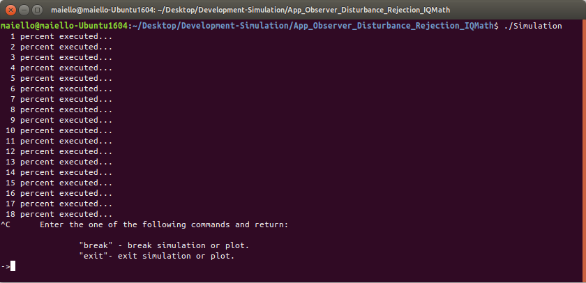
> make clean> make g++ -c -g -no-pie -DUSE_TMP_RAM_DISK -DDEBUGGA ../Simulation/Simulation.cc g++ -c -g -no-pie -DUSE_TMP_RAM_DISK -DDEBUGGA ../Simulation/Application.cc g++ -c -g -no-pie -DUSE_TMP_RAM_DISK -DDEBUGGA ../Simulation/gnuplot_i.cc ../Simulation/gnuplot_i.hpp> ./Simulation
Type “ctrl-c” to stop simulation.
  1 percent executed...
  2 percent executed...
  3 percent executed...
  4 percent executed...
  .
  .
  .
 68 percent executed...
 69 percent executed...
 70 percent executed...
 71 percent executed...
 72 percent executed...
 73 percent executed...
 74 percent executed...
 75 percent executed...
 76 percent executed...
^C	Enter the one of the following commands and return:

		"break" - break simulation or plot.
		"exit"- exit simulation or plot.

  -> break


 Simulation stopped...


	   Current Time - 0.769857
	Simulation Time - 1


	Enter Plot Time Offset followed by
	Plot Name<return>
	Scale factor<return>
	Min Time<return>
	Max Time<return>
	...
	Use symbol "*" to plot ALL or to terminate names.
	Use symbol "$h" to plot time stepping parameter "h".


Plot Offset:
Type “break” and return.
There are six parameters that need to be entered
| Plot offset: | Beginning of displayed plot. (Usually just enter 0 here.) |
| Plot Name | The name of the variable to be plotted. |
| Scale factor | Applied scale factor to variable selected, 1 if unchanged. |
| Min Time | Time beginning of the variable to be plotted offset from 0 time. |
| Max Time | Time ending of the variable to be plotted. |
| Plot Time Step: | Time increment in seconds for which to select successive plot points. Type “0” if you want the points of every time sample plotted. Careful! For simulations that are set for a very a small time sample, this would generate a very large data set. |
Plot offset is entered only one time if multiple variables are to be plotted. The other five parameters are entered for each variable to be plotted. Typing the character “*” for the Plot Name terminates the entry mode and begins the plot process.
In other words, if more than one variable is to be plotted, its name would be entered after Max Time of the previous variable. Otherwise type “*” to start the plotting process.
The plot names are selected by special code placed in the simulation file. There are two ways to select plotting names, object intrinsic and explicit.
Referring to file App_Observer_Disturbance_Rejection_IQMath.hpp
An example for an object intrinsic is
#ifdef RECORD_ALL_PROBES PlotThisOutput = TRUE;#endif Plot_Tag = "TriangleWave";
at line 1303. The Plot Name would be TriangleWave
For an example of explicit
  else if(TagNamesToPlot[i] == "alpha")
	SimuPlot.plot_xy(Plot_t, alpha_a, "alpha");
at line 3151. The Plot Name would be alpha
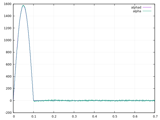
Referring to the paper Brushless AC Motor Control(Disturbance Compensation based on Numerical Modeling) for Figure 8 on page 9, let us plot the variables alpha and alphad.
    Plot Offset:0
    ->alphad
    Scale Factor:1
    Minimum Plot Time:0
    Maximum Plot Time:.7
    Plot Time Step:0
    ->alpha
    Scale Factor:1
    Minimum Plot Time:0
    Maximum Plot Time:.7
    Plot Time Step:0
    ->*
The following plot would be created.
Type “ctrl-c” and type the word exit to end the simulation run.
Finally, for the special code added to the simulation program that creates file fix_double_plot_compare.dat at the end of the simulation, we can use the plot utility gnuplot to plot this data.
Open the gnuplot utility.
gnuplot> set gridgnuplot> set xlabel "Time sample"gnuplot> plot 'fix_double_plot_compare.dat' using 1 with lines title 'ia_m_', '' using 2 with lines title 'ia_m_ fix'
Here, ia_m_ is the calculated double precision value for the current ia and ia_m_fix is the calulated fixed point (32 bit) value for ia.
The generated plot is shown below.
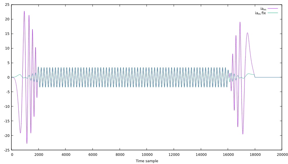
From the plot above there is obviously a tracking issue between the two calculated values during periods of acceleration and deceleration.
The fixed-point solution is in error. The code for the fixed-point calculation is found in file PhyMotorModeSolveFixed.hpp. There may be an error in gaussian elimination setup or the setting of the fixed-point value (statement #define FPT_WBITS 8 at line 3 of this file) may not be set appropriately.
